8. Intro to NumPy and Pandas

8.1. Overview

This lecture introduces NumPy and Pandas, two fundamental libraries for data manipulation and analysis in Python, with applications in geospatial programming. NumPy is essential for numerical operations and handling arrays, while Pandas provides powerful tools for data analysis, particularly when working with tabular data. Understanding these libraries will enable you to perform complex data operations efficiently and effectively in geospatial contexts.

8.2. Learning Objectives

By the end of this lecture, you should be able to:

• Understand the basics of NumPy arrays and how to perform operations on them.

• Utilize Pandas DataFrames to organize, analyze, and manipulate tabular data.

• Apply NumPy and Pandas in geospatial programming to process and analyze geospatial datasets.

• Combine NumPy and Pandas to streamline data processing workflows.

• Develop the ability to perform complex data operations, such as filtering, aggregating, and transforming geospatial data.

8.3. Introduction to NumPy

NumPy (Numerical Python) is a library used for scientific computing. It provides support for large, multi-dimensional arrays and matrices, along with a collection of mathematical functions to operate on these arrays.

8.3.1. Creating NumPy Arrays

Let’s start by creating some basic NumPy arrays.

import numpy as np

# Creating a 1D array
arr_1d = np.array([1, 2, 3, 4, 5])
print(f"1D Array: {arr_1d}")

1D Array: [1 2 3 4 5]

# Creating a 2D array
arr_2d = np.array([[1, 2, 3], [4, 5, 6]])
print(f"2D Array:\n{arr_2d}")

2D Array:
[[1 2 3]
 [4 5 6]]

# Creating an array of zeros
zeros = np.zeros((3, 3))
print(f"Array of zeros:\n{zeros}")

Array of zeros:
[[0. 0. 0.]
 [0. 0. 0.]
 [0. 0. 0.]]

# Creating an array of ones
ones = np.ones((2, 4))
print(f"Array of ones:\n{ones}")

Array of ones:
[[1. 1. 1. 1.]
 [1. 1. 1. 1.]]

# Creating an array with a range of values
range_arr = np.arange(0, 10, 2)
print(f"Range Array: {range_arr}")

Range Array: [0 2 4 6 8]

8.3.2. Basic Array Operations

NumPy allows you to perform element-wise operations on arrays.

# Array addition
arr_sum = arr_1d + 10
print(f"Array after addition: {arr_sum}")

Array after addition: [11 12 13 14 15]

# Array multiplication
arr_product = arr_1d * 2
print(f"Array after multiplication: {arr_product}")

Array after multiplication: [ 2  4  6  8 10]

# Element-wise multiplication of two arrays
arr_2d_product = arr_2d * np.array([1, 2, 3])
print(f"Element-wise multiplication of 2D array:\n{arr_2d_product}")

Element-wise multiplication of 2D array:
[[ 1  4  9]
 [ 4 10 18]]

8.3.3. Reshaping Arrays

Reshaping arrays can be particularly useful when you need to restructure data for specific computations or visualizations.

# Reshape a 1D array into a 2D array
arr_reshaped = np.arange(12).reshape((3, 4))
print(f"Reshaped 1D Array into 2D Array:\n{arr_reshaped}")

Reshaped 1D Array into 2D Array:
[[ 0  1  2  3]
 [ 4  5  6  7]
 [ 8  9 10 11]]

arr_reshaped.shape

(3, 4)

8.3.4. Mathematical Functions on Arrays

You can apply various mathematical functions to arrays, such as square roots, logarithms, and trigonometric functions.

# Square root of each element in the array
sqrt_array = np.sqrt(arr_reshaped)
print(f"Square Root of Array Elements:\n{sqrt_array}")

Square Root of Array Elements:
[[0.         1.         1.41421356 1.73205081]
 [2.         2.23606798 2.44948974 2.64575131]
 [2.82842712 3.         3.16227766 3.31662479]]

# Logarithm of each element (add 1 to avoid log(0))
log_array = np.log1p(arr_reshaped)
print(f"Logarithm (base e) of Array Elements:\n{log_array}")

Logarithm (base e) of Array Elements:
[[0.         0.69314718 1.09861229 1.38629436]
 [1.60943791 1.79175947 1.94591015 2.07944154]
 [2.19722458 2.30258509 2.39789527 2.48490665]]

8.3.5. Statistical Operations

NumPy provides a wide range of statistical functions for data analysis, such as mean, median, variance, and standard deviation.

# Mean, median, and standard deviation of an array
arr = np.array([1, 2, 3, 4, 5, 6, 7, 8, 9, 10])
mean_val = np.mean(arr)
median_val = np.median(arr)
std_val = np.std(arr)

print(f"Mean: {mean_val}, Median: {median_val}, Standard Deviation: {std_val:.4f}")

Mean: 5.5, Median: 5.5, Standard Deviation: 2.8723

8.3.6. Random Data Generation for Simulation

Random data generation is useful for simulations, such as generating random geospatial coordinates or sampling from distributions.

# Generate an array of random latitudes and longitudes
random_coords = np.random.uniform(low=-90, high=90, size=(5, 2))
print(f"Random Latitudes and Longitudes:\n{random_coords}")

Random Latitudes and Longitudes:
[[  1.6884375   -0.58090868]
 [ 43.93093834  11.96520412]
 [-85.25180701  63.83221312]
 [-82.38763071  85.80113984]
 [-25.60998373  71.21172342]]

8.3.7. Indexing, Slicing, and Iterating

One of the most powerful features of NumPy is its ability to quickly access and modify array elements using indexing and slicing. These operations allow you to select specific parts of the array, which is useful in many geospatial applications where you may want to work with subsets of your data (e.g., focusing on specific regions or coordinates).

8.3.7.1. Indexing in NumPy

You can access individual elements of an array using their indices. Remember that NumPy arrays are zero-indexed, meaning that the first element is at index 0.

Below are some examples of indexing 1D Arrays in NumPy.

# Create a 1D array
arr = np.array([10, 20, 30, 40, 50])

# Accessing the first element
first_element = arr[0]
print(f"First element: {first_element}")

# Accessing the last element
last_element = arr[-1]
print(f"Last element: {last_element}")

First element: 10
Last element: 50

In 2D arrays, you can specify both row and column indices to access a particular element.

# Create a 2D array
arr_2d = np.array([[1, 2, 3], [4, 5, 6], [7, 8, 9]])
arr_2d

array([[1, 2, 3],
       [4, 5, 6],
       [7, 8, 9]])

# Accessing the element in the first row and second column
element = arr_2d[0, 1]
print(f"Element at row 1, column 2: {element}")

# Accessing the element in the last row and last column
element_last = arr_2d[-1, -1]
print(f"Element at last row, last column: {element_last}")

Element at row 1, column 2: 2
Element at last row, last column: 9

8.3.7.2. Slicing in NumPy

Slicing allows you to access a subset of an array. You can use the : symbol to specify a range of indices.

Example: Slicing 1D Arrays in NumPy

# Create a 1D array
arr = np.array([10, 20, 30, 40, 50])

# Slice elements from index 1 to 3 (exclusive)
slice_1d = arr[1:4]
print(f"Slice from index 1 to 3: {slice_1d}")

# Slice all elements from index 2 onwards
slice_2d = arr[2:]
print(f"Slice from index 2 onwards: {slice_2d}")

Slice from index 1 to 3: [20 30 40]
Slice from index 2 onwards: [30 40 50]

Example: Slicing 2D Arrays in NumPy

When slicing a 2D array, you can slice both rows and columns.

# Create a 2D array
arr_2d = np.array([[1, 2, 3], [4, 5, 6], [7, 8, 9]])
arr_2d

array([[1, 2, 3],
       [4, 5, 6],
       [7, 8, 9]])

# Slice the first two rows and all columns
slice_2d = arr_2d[:2, :]
print(f"Sliced 2D array (first two rows):\n{slice_2d}")

# Slice the last two rows and the first two columns
slice_2d_partial = arr_2d[1:, :2]
print(f"Sliced 2D array (last two rows, first two columns):\n{slice_2d_partial}")

Sliced 2D array (first two rows):
[[1 2 3]
 [4 5 6]]
Sliced 2D array (last two rows, first two columns):
[[4 5]
 [7 8]]

8.3.7.3. Boolean Indexing

You can also use Boolean conditions to filter elements of an array.

Example: Boolean Indexing

# Create a 1D array
arr = np.array([10, 20, 30, 40, 50])

# Boolean condition to select elements greater than 25
condition = arr > 25
print(f"Boolean condition: {condition}")

# Use the condition to filter the array
filtered_arr = arr[condition]
print(f"Filtered array (elements > 25): {filtered_arr}")

Boolean condition: [False False  True  True  True]
Filtered array (elements > 25): [30 40 50]

8.3.7.4. Iterating Over Arrays

You can iterate over NumPy arrays to access or modify elements. For 1D arrays, you can simply loop through the elements. For multi-dimensional arrays, you may want to iterate through rows or columns.

Example: Iterating Over a 1D Array

# Create a 1D array
arr = np.array([10, 20, 30, 40, 50])

# Iterating through the array
for element in arr:
    print(f"Element: {element}")

Element: 10
Element: 20
Element: 30
Element: 40
Element: 50

Example: Iterating Over a 2D Array

# Create a 2D array
arr_2d = np.array([[1, 2, 3], [4, 5, 6], [7, 8, 9]])

# Iterating through rows of the 2D array
print("Iterating over rows:")
for row in arr_2d:
    print(row)

# Iterating through each element of the 2D array
print("\nIterating over each element:")
for row in arr_2d:
    for element in row:
        print(element, end=" ")

Iterating over rows:
[1 2 3]
[4 5 6]
[7 8 9]

Iterating over each element:
1 2 3 4 5 6 7 8 9 

8.3.8. Modifying Array Elements

You can also use indexing and slicing to modify elements of the array.

Example: Modifying Elements

# Create a 1D array
arr = np.array([10, 20, 30, 40, 50])

# Modify the element at index 1
arr[1] = 25
print(f"Modified array: {arr}")

# Modify multiple elements using slicing
arr[2:4] = [35, 45]
print(f"Modified array with slicing: {arr}")

Modified array: [10 25 30 40 50]
Modified array with slicing: [10 25 35 45 50]

8.3.9. Working with Geospatial Coordinates

You can use NumPy to perform calculations on arrays of geospatial coordinates, such as converting from degrees to radians.

# Array of latitudes and longitudes
coords = np.array([[35.6895, 139.6917], [34.0522, -118.2437], [51.5074, -0.1278]])

# Convert degrees to radians
coords_radians = np.radians(coords)
print(f"Coordinates in radians:\n{coords_radians}")

Coordinates in radians:
[[ 6.22899283e-01  2.43808010e+00]
 [ 5.94323008e-01 -2.06374188e+00]
 [ 8.98973719e-01 -2.23053078e-03]]

8.4. Introduction to Pandas

Pandas is a powerful data manipulation library that provides data structures like Series and DataFrames to work with structured data. It is especially useful for handling tabular data.

8.4.1. Creating Pandas Series and DataFrames

Let’s create a Pandas Series and DataFrame. Each column in a DataFrame is a Series.

import pandas as pd

# Creating a Series
city_series = pd.Series(["Tokyo", "Los Angeles", "London"], name="City")
print(f"Pandas Series:\n{city_series}\n")

Pandas Series:
0          Tokyo
1    Los Angeles
2         London
Name: City, dtype: object

# Creating a DataFrame
data = {
    "City": ["Tokyo", "Los Angeles", "London"],
    "Latitude": [35.6895, 34.0522, 51.5074],
    "Longitude": [139.6917, -118.2437, -0.1278],
}
df = pd.DataFrame(data)
print(f"Pandas DataFrame:\n{df}")

Pandas DataFrame:
          City  Latitude  Longitude
0        Tokyo   35.6895   139.6917
1  Los Angeles   34.0522  -118.2437
2       London   51.5074    -0.1278

df

	City	Latitude	Longitude
0	Tokyo	35.6895	139.6917
1	Los Angeles	34.0522	-118.2437
2	London	51.5074	-0.1278

8.4.2. Basic DataFrame Operations

You can perform various operations on Pandas DataFrames, such as filtering, selecting specific columns, and applying functions.

# Selecting a specific column
latitudes = df["Latitude"]
print(f"Latitudes:\n{latitudes}\n")

Latitudes:
0    35.6895
1    34.0522
2    51.5074
Name: Latitude, dtype: float64

# Filtering rows based on a condition
df_filtered = df[df["Longitude"] < 0]
df_filtered

	City	Latitude	Longitude
1	Los Angeles	34.0522	-118.2437
2	London	51.5074	-0.1278

# Adding a new column with a calculation
df["Lat_Radians"] = np.radians(df["Latitude"])
df

	City	Latitude	Longitude	Lat_Radians
0	Tokyo	35.6895	139.6917	0.622899
1	Los Angeles	34.0522	-118.2437	0.594323
2	London	51.5074	-0.1278	0.898974

8.4.3. Grouping and Aggregation

Pandas allows you to group data and perform aggregate functions, which is useful in summarizing large datasets.

# Creating a DataFrame
data = {
    "City": ["Tokyo", "Los Angeles", "London", "Paris", "Chicago"],
    "Country": ["Japan", "USA", "UK", "France", "USA"],
    "Population": [37400068, 3970000, 9126366, 2140526, 2665000],
}
df = pd.DataFrame(data)
df

	City	Country	Population
0	Tokyo	Japan	37400068
1	Los Angeles	USA	3970000
2	London	UK	9126366
3	Paris	France	2140526
4	Chicago	USA	2665000

# Group by 'Country' and calculate the total population for each country
df_grouped = df.groupby("Country")["Population"].sum()
print(f"Total Population by Country:\n{df_grouped}")

Total Population by Country:
Country
France     2140526
Japan     37400068
UK         9126366
USA        6635000
Name: Population, dtype: int64

8.4.4. Merging DataFrames

Merging datasets is essential when combining different geospatial datasets, such as joining city data with demographic information.

# Creating two DataFrames to merge
df1 = pd.DataFrame(
    {"City": ["Tokyo", "Los Angeles", "London"], "Country": ["Japan", "USA", "UK"]}
)
df2 = pd.DataFrame(
    {
        "City": ["Tokyo", "Los Angeles", "London"],
        "Population": [37400068, 3970000, 9126366],
    }
)

df1

	City	Country
0	Tokyo	Japan
1	Los Angeles	USA
2	London	UK

df2

	City	Population
0	Tokyo	37400068
1	Los Angeles	3970000
2	London	9126366

# Merge the two DataFrames on the 'City' column
df_merged = pd.merge(df1, df2, on="City")
df_merged

	City	Country	Population
0	Tokyo	Japan	37400068
1	Los Angeles	USA	3970000
2	London	UK	9126366

8.4.5. Handling Missing Data

In real-world datasets, missing data is common. Pandas provides tools to handle missing data, such as filling or removing missing values.

# Creating a DataFrame with missing values
data_with_nan = {
    "City": ["Tokyo", "Los Angeles", "London", "Paris"],
    "Population": [37400068, 3970000, None, 2140526],
}
df_nan = pd.DataFrame(data_with_nan)
df_nan

	City	Population
0	Tokyo	37400068.0
1	Los Angeles	3970000.0
2	London	NaN
3	Paris	2140526.0

# Fill missing values with the mean population
df_filled = df_nan.fillna(df_nan["Population"].mean())
df_filled

	City	Population
0	Tokyo	3.740007e+07
1	Los Angeles	3.970000e+06
2	London	1.450353e+07
3	Paris	2.140526e+06

8.4.6. Reading Geospatial Data from a CSV File

Pandas can read and write data in various formats, such as CSV, Excel, and SQL databases. This makes it easy to load and save data from different sources. For example, you can read a CSV file into a Pandas DataFrame and then perform operations on the data.

Let’s read a CSV file from an HTTP URL into a Pandas DataFrame and display the first few rows of the data.

url = "https://github.com/opengeos/datasets/releases/download/world/world_cities.csv"
df = pd.read_csv(url)
df.head()

	id	name	country	latitude	longitude	population
0	1	Bombo	UGA	0.5833	32.5333	75000
1	2	Fort Portal	UGA	0.6710	30.2750	42670
2	3	Potenza	ITA	40.6420	15.7990	69060
3	4	Campobasso	ITA	41.5630	14.6560	50762
4	5	Aosta	ITA	45.7370	7.3150	34062

The DataFrame contains information about world cities, including their names, countries, populations, and geographical coordinates. We can calculate the total population of all cities in the dataset using NumPy and Pandas as follows.

np.sum(df["population"])

1475534501

8.4.7. Creating plots with Pandas

Pandas provides built-in plotting capabilities that allow you to create various types of plots directly from DataFrames.

# Load the dataset from an online source
url = "https://raw.githubusercontent.com/pandas-dev/pandas/main/doc/data/air_quality_no2.csv"
air_quality = pd.read_csv(url, index_col=0, parse_dates=True)

# Display the first few rows of the dataset
air_quality.head()

	station_antwerp	station_paris	station_london
datetime
2019-05-07 02:00:00	NaN	NaN	23.0
2019-05-07 03:00:00	50.5	25.0	19.0
2019-05-07 04:00:00	45.0	27.7	19.0
2019-05-07 05:00:00	NaN	50.4	16.0
2019-05-07 06:00:00	NaN	61.9	NaN

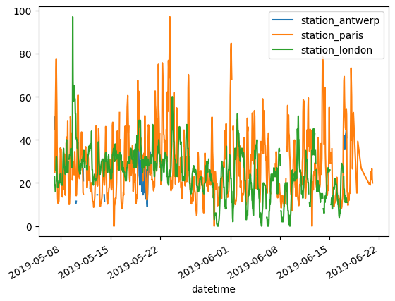
To do a quick visual check of the data.

air_quality.plot()

<Axes: xlabel='datetime'>

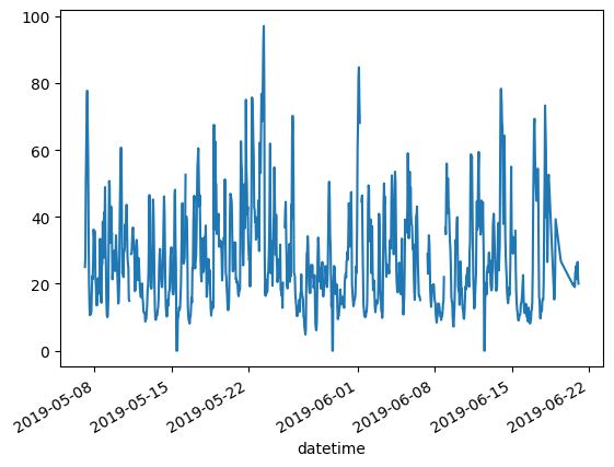
To plot only the columns of the data table with the data from Paris.

air_quality["station_paris"].plot()

<Axes: xlabel='datetime'>

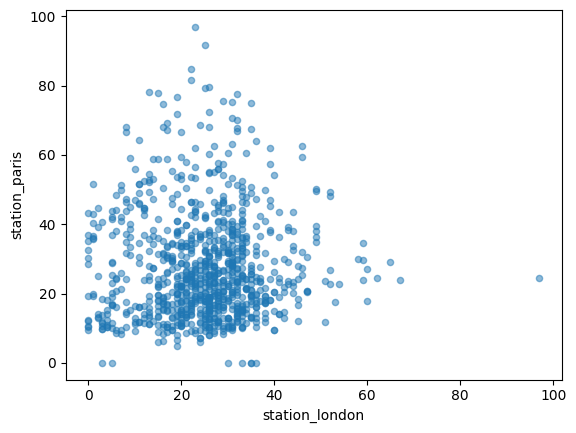
To visually compare the values measured in London versus Paris.

air_quality.plot.scatter(x="station_london", y="station_paris", alpha=0.5)

<Axes: xlabel='station_london', ylabel='station_paris'>

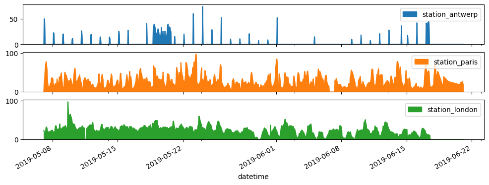
To visualize each of the columns in a separate subplot.

air_quality.plot.area(figsize=(12, 4), subplots=True)

array([<Axes: xlabel='datetime'>, <Axes: xlabel='datetime'>,
       <Axes: xlabel='datetime'>], dtype=object)

8.4.8. Analyzing Geospatial Data

In this example, we analyze a dataset of cities, calculating the distance between each pair using the Haversine formula.

# Define the Haversine formula using NumPy
def haversine_np(lat1, lon1, lat2, lon2):
    R = 6371.0  # Earth radius in kilometers
    dlat = np.radians(lat2 - lat1)
    dlon = np.radians(lon2 - lon1)
    a = (
        np.sin(dlat / 2) ** 2
        + np.cos(np.radians(lat1)) * np.cos(np.radians(lat2)) * np.sin(dlon / 2) ** 2
    )
    c = 2 * np.arctan2(np.sqrt(a), np.sqrt(1 - a))
    distance = R * c
    return distance


# Create a new DataFrame with city pairs
city_pairs = pd.DataFrame(
    {
        "City1": ["Tokyo", "Tokyo", "Los Angeles"],
        "City2": ["Los Angeles", "London", "London"],
        "Lat1": [35.6895, 35.6895, 34.0522],
        "Lon1": [139.6917, 139.6917, -118.2437],
        "Lat2": [34.0522, 51.5074, 51.5074],
        "Lon2": [-118.2437, -0.1278, -0.1278],
    }
)
city_pairs

	City1	City2	Lat1	Lon1	Lat2	Lon2
0	Tokyo	Los Angeles	35.6895	139.6917	34.0522	-118.2437
1	Tokyo	London	35.6895	139.6917	51.5074	-0.1278
2	Los Angeles	London	34.0522	-118.2437	51.5074	-0.1278

# Calculate distances between city pairs
city_pairs["Distance_km"] = haversine_np(
    city_pairs["Lat1"], city_pairs["Lon1"], city_pairs["Lat2"], city_pairs["Lon2"]
)
city_pairs

	City1	City2	Lat1	Lon1	Lat2	Lon2	Distance_km
0	Tokyo	Los Angeles	35.6895	139.6917	34.0522	-118.2437	8815.473356
1	Tokyo	London	35.6895	139.6917	51.5074	-0.1278	9558.713695
2	Los Angeles	London	34.0522	-118.2437	51.5074	-0.1278	8755.602341

8.5. Combining NumPy and Pandas

You can combine NumPy and Pandas to perform complex data manipulations. For instance, you might want to apply NumPy functions to a Pandas DataFrame or use Pandas to organize and visualize the results of NumPy operations.

Let’s say you have a dataset of cities, and you want to calculate the average distance from each city to all other cities.

# Define a function to calculate distances from a city to all other cities
def calculate_average_distance(df):
    lat1 = df["Latitude"].values
    lon1 = df["Longitude"].values
    lat2, lon2 = np.meshgrid(lat1, lon1)
    distances = haversine_np(lat1, lon1, lat2, lon2)
    avg_distances = np.mean(distances, axis=1)
    return avg_distances


# Creating a DataFrame
data = {
    "City": ["Tokyo", "Los Angeles", "London"],
    "Latitude": [35.6895, 34.0522, 51.5074],
    "Longitude": [139.6917, -118.2437, -0.1278],
}
df = pd.DataFrame(data)

# Apply the function to calculate average distances
df["Avg_Distance_km"] = calculate_average_distance(df)
df

	City	Latitude	Longitude	Avg_Distance_km
0	Tokyo	35.6895	139.6917	5624.601390
1	Los Angeles	34.0522	-118.2437	5294.682354
2	London	51.5074	-0.1278	7041.924003

8.6. Exercises

1. Array Operations: Create a NumPy array representing the elevations of various locations. Normalize the elevations (e.g., subtract the mean and divide by the standard deviation) and calculate the mean and standard deviation of the normalized array.

2. Data Analysis with Pandas: Create a Pandas DataFrame from a CSV file containing geospatial data (e.g., cities and their coordinates). Filter the DataFrame to include only cities in the Northern Hemisphere and calculate the average latitude of these cities.

3. Combining NumPy and Pandas: Using a dataset of geographic coordinates, create a Pandas DataFrame. Use NumPy to calculate the pairwise distances between all points and store the results in a new DataFrame.

8.7. Summary

NumPy and Pandas are essential tools in geospatial programming, allowing you to efficiently manipulate and analyze numerical and tabular data. By mastering these libraries, you will be able to perform complex data operations, manage large datasets, and streamline your geospatial workflows.