Xarray

12. Xarray#

12.1. Overview#

Xarray is a powerful Python library designed for working with multi-dimensional labeled datasets, often used in fields such as climate science, oceanography, and remote sensing. It provides a high-level interface for manipulating and analyzing datasets that can be thought of as extensions of NumPy arrays. Xarray is particularly useful for geospatial data because it supports labeled axes (dimensions), coordinates, and metadata, making it easier to work with datasets that vary across time, space, and other dimensions.

12.2. Learning Objectives#

By the end of this lecture, you should be able to:

Understand the basic concepts and data structures in Xarray, including DataArray and Dataset.
Load and inspect multi-dimensional geospatial datasets using Xarray.
Perform basic operations on Xarray objects, such as selection, indexing, and arithmetic operations.
Use Xarray to efficiently work with large geospatial datasets, including time series and raster data.
Apply Xarray to common geospatial analysis tasks, such as calculating statistics, regridding, and visualization.

12.3. What is Xarray?#

Xarray extends the capabilities of NumPy by providing a data structure for labeled, multi-dimensional arrays. The two main data structures in Xarray are:

DataArray: A labeled, multi-dimensional array, which includes dimensions, coordinates, and attributes.
Dataset: A collection of DataArray objects that share the same dimensions.

Xarray is particularly useful for working with datasets where dimensions have meaningful labels (e.g., time, latitude, longitude) and where metadata is important.

12.4. Installing Xarray#

Before we start, ensure that Xarray is installed. You can install it via pip:

# %pip install xarray pooch

12.5. Importing Libraries#

import matplotlib.pyplot as plt
import numpy as np
import xarray as xr

xr.set_options(keep_attrs=True, display_expand_data=False)
np.set_printoptions(threshold=10, edgeitems=2)

12.6. Xarray Data Structures#

Xarray provides two core data structures:

DataArray: A single multi-dimensional array with labeled dimensions, coordinates, and metadata.
Dataset: A collection of DataArray objects, each corresponding to a variable, sharing the same dimensions and coordinates.

12.9. DataArray Components#

Values: The actual data stored in a NumPy array or similar structure.
Dimensions: Named axes of the data (e.g., time, latitude, longitude).
Coordinates: Labels for the values in each dimension (e.g., specific times or geographic locations).
Attributes: Metadata associated with the data (e.g., units, descriptions).

You can extract and print the values, dimensions, and coordinates of a DataArray:

temperature.values

array([[[241.2 , 242.5 , ..., 235.5 , 238.6 ],
        [243.8 , 244.5 , ..., 235.3 , 239.3 ],
        ...,
        [295.9 , 296.2 , ..., 295.9 , 295.2 ],
        [296.29, 296.79, ..., 296.79, 296.6 ]],

       [[242.1 , 242.7 , ..., 233.6 , 235.8 ],
        [243.6 , 244.1 , ..., 232.5 , 235.7 ],
        ...,
        [296.2 , 296.7 , ..., 295.5 , 295.1 ],
        [296.29, 297.2 , ..., 296.4 , 296.6 ]],

       ...,

       [[245.79, 244.79, ..., 243.99, 244.79],
        [249.89, 249.29, ..., 242.49, 244.29],
        ...,
        [296.29, 297.19, ..., 295.09, 294.39],
        [297.79, 298.39, ..., 295.49, 295.19]],

       [[245.09, 244.29, ..., 241.49, 241.79],
        [249.89, 249.29, ..., 240.29, 241.69],
        ...,
        [296.09, 296.89, ..., 295.69, 295.19],
        [297.69, 298.09, ..., 296.19, 295.69]]])

temperature.dims

('time', 'lat', 'lon')

temperature.coords

Coordinates:
  * lat      (lat) float32 100B 75.0 72.5 70.0 67.5 65.0 ... 22.5 20.0 17.5 15.0
  * lon      (lon) float32 212B 200.0 202.5 205.0 207.5 ... 325.0 327.5 330.0
  * time     (time) datetime64[ns] 23kB 2013-01-01 ... 2014-12-31T18:00:00

temperature.attrs

{'long_name': '4xDaily Air temperature at sigma level 995',
 'units': 'degK',
 'precision': np.int16(2),
 'GRIB_id': np.int16(11),
 'GRIB_name': 'TMP',
 'var_desc': 'Air temperature',
 'dataset': 'NMC Reanalysis',
 'level_desc': 'Surface',
 'statistic': 'Individual Obs',
 'parent_stat': 'Other',
 'actual_range': array([185.16, 322.1 ], dtype=float32)}

12.12. Visualization with Xarray#

Xarray integrates well with Matplotlib and other visualization libraries, making it easy to create plots directly from DataArray and Dataset objects.

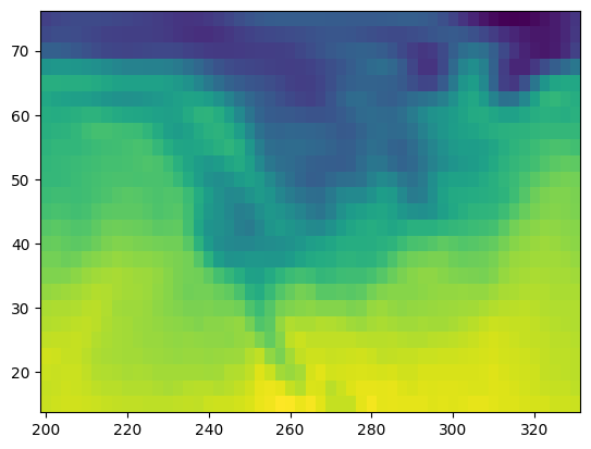
# Plot the mean temperature
mean_temperature.plot()
plt.show()

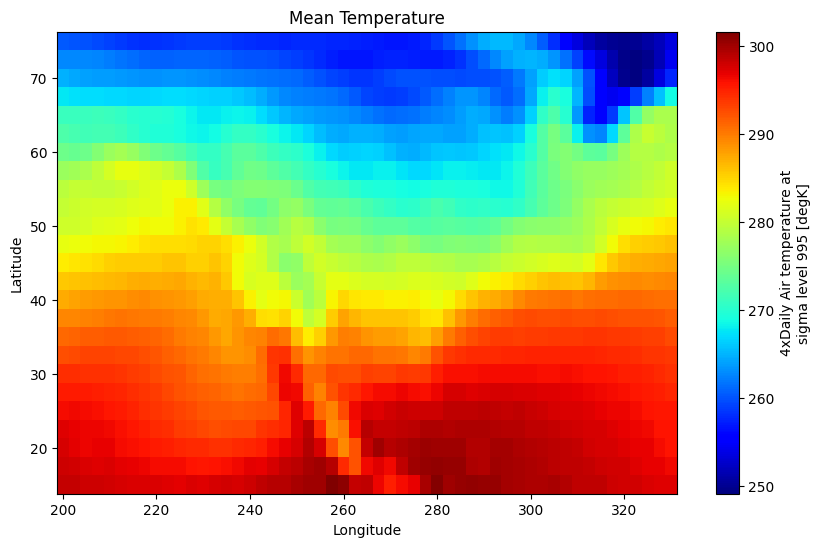
../../_images/01e415b0bd171b159030ff9c9e1255958d0667c759d342dde8fccf6a1b041d0d.png

You can customize the appearance of plots by passing arguments to the plot method. For example, you can specify the color map, add labels, and set the figure size.

mean_temperature.plot(cmap="jet", figsize=(10, 6))
plt.xlabel("Longitude")
plt.ylabel("Latitude")
plt.title("Mean Temperature")

Text(0.5, 1.0, 'Mean Temperature')

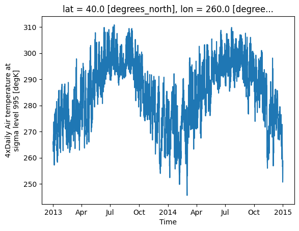
../../_images/56775802710fd14c80f6453efaf621f30b429233bf828cb9de79f9d92ee2880b.png

You can also select a specific location using the sel method and plot a time series of temperature at that location.

# Plot a time series for a specific location
temperature.sel(lat=40.0, lon=260.0).plot()
plt.show()

../../_images/0bbd51a9b82b90b0364633d6de754f5b8e0f09081b869b545105410d47f6f056.png

12.14. Why Use Xarray?#

Xarray is valuable for handling multi-dimensional data, especially in scientific applications. It provides metadata, dimension names, and coordinate labels, making it much easier to understand and manipulate data compared to raw NumPy arrays.

12.14.1. Without Xarray (Using NumPy)#

Here’s how a task might look without Xarray, using NumPy arrays:

lat = ds.air.lat.data
lon = ds.air.lon.data
temp = ds.air.data

temp.shape

(2920, 25, 53)

plt.figure()
plt.pcolormesh(lon, lat, temp[0, :, :])

<matplotlib.collections.QuadMesh at 0x7f930dc786e0>

../../_images/6f22a45aceea1603970dffd90e49785bd6c7ac2c0cd389750d9db81af6266002.png

While this approach works, it’s not clear what 0 refers to (in this case, it’s the first time step).

12.14.2. With Xarray#

With Xarray, you can use more intuitive and readable indexing with sel and isel:

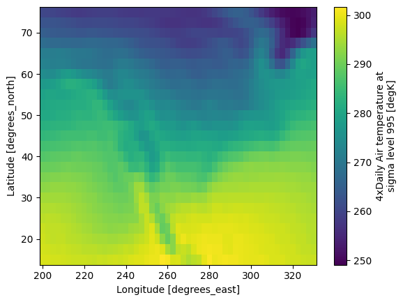
ds.air.isel(time=0).plot(x="lon")

<matplotlib.collections.QuadMesh at 0x7f930dc7a900>

../../_images/5175a33104c01e3f7b4a1fd979100d3b328f5c7833965e5db963af9b0a365c71.png

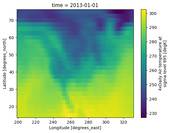
ds.air.sel(time="2013-01-01T00:00:00").plot(x="lon")

<matplotlib.collections.QuadMesh at 0x7f930db64650>

This example selects the first time step and plots it using labeled axes (lat and lon), which is much clearer.

12.16. High-Level Computations with Xarray#

Xarray offers several high-level operations that make common computations straightforward, such as groupby, resample, rolling, and weighted.

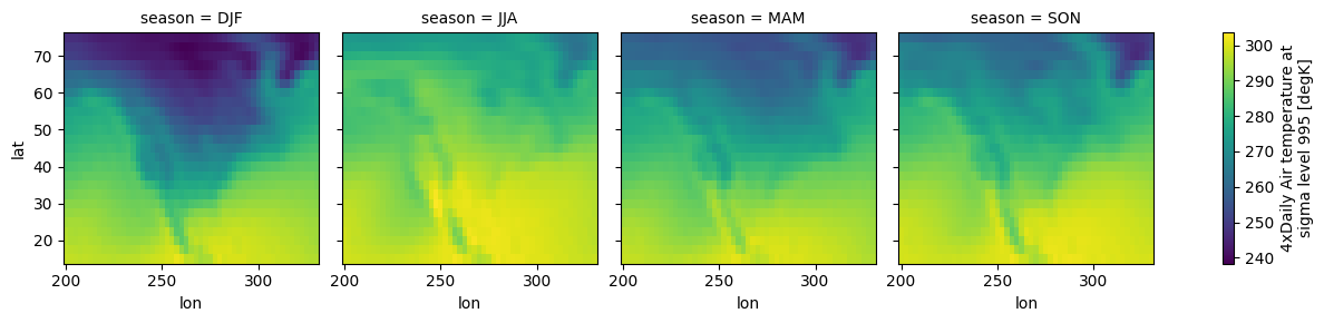
12.16.1. GroupBy Operation#

You can calculate statistics such as the seasonal mean of the dataset:

seasonal_mean = ds.groupby("time.season").mean()
seasonal_mean.air.plot(col="season")

<xarray.plot.facetgrid.FacetGrid at 0x7f930da9fef0>

../../_images/15302f7427fd458a1917f31397518b085ec0f7e70ac29e62d8124c110dc259e6.png

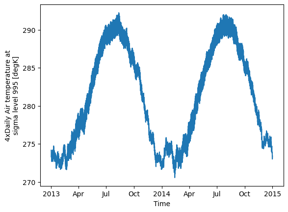
12.16.2. Computation with Weights#

Xarray allows for weighted computations, useful in geospatial contexts where grid cells vary in size. For example, you can weight the mean of the dataset by cell area.

cell_area = xr.ones_like(ds.air.lon)  # Placeholder for actual area calculation
weighted_mean = ds.weighted(cell_area).mean(dim=["lon", "lat"])
weighted_mean.air.plot()

[<matplotlib.lines.Line2D at 0x7f930da86c00>]

../../_images/10f99c0bb3e851ba6c198a19a8a162f5219073f80a132f5276dddd258bfbf267.png

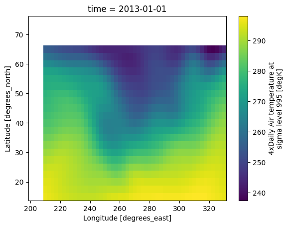
12.16.3. Rolling Window Operation#

Xarray supports rolling window operations, which are useful for smoothing time series data spatially or temporally. For example, you can smooth the temperature data spatially using a 5x5 window.

ds.air.isel(time=0).rolling(lat=5, lon=5).mean().plot()

<matplotlib.collections.QuadMesh at 0x7f930d84cb60>

../../_images/ca550f25bee926dbeed9279cfcd9ab5bb3c53713e74ae02c369b9ed17679c914.png

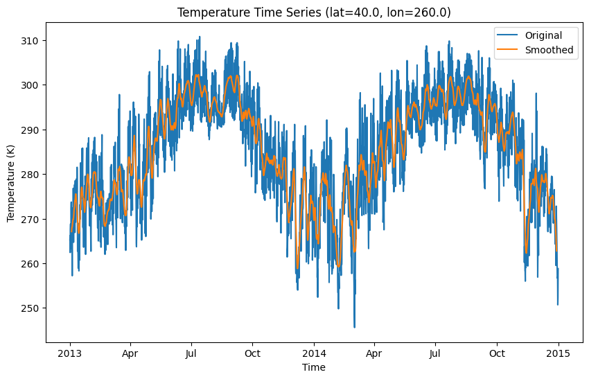
Similarly, you can smooth the temperature data temporally using a 5-day window.

plt.figure(figsize=(10, 6))
# Select the time series at a specific latitude and longitude
temperature = ds["air"].sel(lat=40.0, lon=260.0)

# Plot the original time series
temperature.plot(label="Original")

# Apply rolling mean smoothing with a window size of 20
smoothed_temperature = temperature.rolling(time=20, center=True).mean()

# Plot the smoothed data
smoothed_temperature.plot(label="Smoothed")

# Add a title and labels
plt.title("Temperature Time Series (lat=40.0, lon=260.0)")
plt.xlabel("Time")
plt.ylabel("Temperature (K)")

# Add a legend
plt.legend()

# Show the plot
plt.show()

../../_images/197cce2e42b47cd64929c01e8e595c3b06baee84dae320c717401160f286a2db.png

12.18. Exercises#

12.18.1. Exercise 1: Exploring a New Dataset#

Load the Xarray tutorial dataset rasm.
Inspect the Dataset object and list all the variables and dimensions.
Select the Tair variable (air temperature).
Print the attributes, dimensions, and coordinates of Tair.

12.18.2. Exercise 2: Data Selection and Indexing#

Select a subset of the Tair data for the date 1980-07-01 and latitude 70.0.
Create a time slice for the entire latitude range between January and March of 1980.
Plot the selected time slice as a line plot.

12.18.3. Exercise 3: Performing Arithmetic Operations#

Compute the mean of the Tair data over the time dimension.
Subtract the computed mean from the original Tair dataset to get the temperature anomalies.
Plot the mean temperature and the anomalies on separate plots.

12.18.4. Exercise 4: GroupBy and Resampling#

Use groupby to calculate the seasonal mean temperature (Tair).
Use resample to calculate the monthly mean temperature for 1980.
Plot the seasonal mean for each season and the monthly mean.

12.18.5. Exercise 5: Writing Data to netCDF#

Select the temperature anomalies calculated in Exercise 3.
Convert the Tair variable to float32 to optimize file size.
Write the anomalies data to a new netCDF file named tair_anomalies.nc.
Load the data back from the file and print its contents.

12.19. Summary#

Xarray is a powerful library for working with multi-dimensional geospatial data. It simplifies data handling by offering labeled dimensions and coordinates, enabling intuitive operations and making analysis more transparent. Xarray’s ability to work seamlessly with NumPy, Dask, and Pandas makes it an essential tool for geospatial and scientific analysis. With Xarray, you can efficiently manage and analyze large, complex datasets, making it a valuable asset for researchers and developers alike.

Xarray

Contents

12. Xarray#

12.1. Overview#

12.2. Learning Objectives#

12.3. What is Xarray?#

12.4. Installing Xarray#

12.5. Importing Libraries#

12.6. Xarray Data Structures#

12.7. Loading a Dataset#

12.8. Working with DataArrays#

12.9. DataArray Components#

12.10. Indexing and Selecting Data#

12.11. Performing Operations on DataArrays#

12.12. Visualization with Xarray#

12.13. Working with Datasets#